Section 5.2 Random Variables
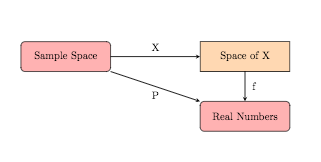
For a given set of events, we might have difficulty doing mathematics since the outcomes are not numerical. In order to accomodate our desire to convert to numerical measures we want to assign numerical values to all outcomes. The process of doing this creates what is known as a random variable.
Definition 5.2.1. Random Variable.
Given a random experiment with sample space \(S\text{,}\) a function \(X\) mapping each element of \(S\) to a unique real number is called a random variable. For each element s from the sample space \(S\text{,}\) denote this function by
\begin{equation*}
X(s) = x
\end{equation*}
and let \(R\) be the range of \(X.\)
\(R\) will be called "the space of X" and in notation
\begin{equation*}
R = { x : X(s)=x, \text{for some} s \in S } .
\end{equation*}
We will make various restrictions on the range of the
random variable 5.2.1 to fit different generalized problems. Then, we will be able to work on a problem (which may be inherently non-numerical) by using the random variable in subsequent calculations.
Example 5.2.2. Success vs Failure.
When dealing with only two outcomes, one might use
\begin{equation*}
S = \text{{ success, failure }}.
\end{equation*}
Choose
\begin{gather*}
X( \text{success})=1\\
X( \text{failure})=0.
\end{gather*}
Then, \(R\) = {0,1}.
Example 5.2.3. Standard Dice Pairs.
When gambling with a pair of dice, one might use S=ordered pairs of all possible rolls. Then
\begin{equation*}
S = \text{ {(a,b): a=die 1 outcome, b=die 2 outcome}}.
\end{equation*}
Choose
\begin{equation*}
X( (a,b) ) = a+b.
\end{equation*}
Then, \(R\) = {2, 3, 4, 5, ..., 12}.
Example 5.2.4. Other Dice Options.
When rolling dice in a board game (like RISK), one might use
\begin{equation*}
S= \text{{ (a,b) : a=die 1 outcome, b=die 2 outcome}}
\end{equation*}
Choose
\begin{equation*}
X( (a,b) ) = \text{max{a,b}}.
\end{equation*}
Then, \(R\) = {1, 2, 3, 4, 5, 6}.
Definition 5.2.5. Countable and Uncountable Sets.
\(R\) contains a countable number of points if either \(R\) is finite or there is a one to one correspondence between R and the positive integers. Such a set will be called discrete. We will see that often the set \(R\) is not countable. If \(R\) consists of an interval of points (or a union of intervals), then we call X a continuous random variable.
Notice that in each of the examples above, the space \(R\) was finite. Therefore, each of those random variables would be considered countable. One can however have random variables with a infinite number of values in \(R\) and yet still be countable.
Example 5.2.6.
Consider the random variable \(X\) representing the number of coin flips until you get a Heads. Even though it is unlikely to have to keep on going, consider the fact that you could continually flip and get Tails every time for a long time. So, the possible values for \(X\) would be \(R\) = {1, 2, 3, 4, ... } which is precisely the infinite set of positive integers. Therefore, \(X\) is a countable random variable.
Example 5.2.7.
Consider the random variable \(X\) representing the time until a light bulb fails to work after being successfully turned on. Notice that the bulb could fail in a relatively short time (near 0 let’s say) or could continue to last for almost eternity (or as long as you might want to measure). However, time is measured on a continuum and therefore for this random variable \(X\) you would have \(R\) equal to the interval from 0 to infinity, i.e. \(R = (0,\infty)\) which is not a countable set.

