The Normal Distribution

Section 9.2 The Normal Distribution

Definition 9.2.1. The Normal Distribution.

Given two parameters

μ

and

σ,

a random variable X over

R = (- \infty, \infty)

has a normal distribution provided it has a probability function given by

f (x) = \frac{1}{σ \sqrt{2 π}} e^{- {(\frac{x - μ}{σ})}^{2} / 2}

🔗

The normal distribution is also sometimes referred to as the Gaussian Distribution (often by Physicists) or the Bell Curve (often by social scientists).


    
        
xxxxxxxxxx
 
1
var('x,mu,sigma')
2
f(x) = e^(-((x-mu)/sigma)^2/2)/(sigma*sqrt(2*pi))
3
@interact
4
def _(m=slider(-10,10,1,0,label='$$\\mu$$'),
5
      s=slider(1/5,5,1/10,1,label='$$\\sigma$$')):
6
    titletext = ("Normal Curve with mean "+
7
          str(m)+" and standard deviation "+str(s))
8
    G = plot(f(mu=m,sigma=s),(x,m-5*s,m+5*s))
9
    G += point((0,1),size=1)+point((12,0),size=1)+point((-12,0),size=1)
10
    G += point((m,f(x=m,mu=m,sigma=s)),color='red',size=20)
11
    G += point((m+s,f(x=m+s,mu=m,sigma=s)),color='green',size=20)
12
    G += point((m-s,f(x=m-s,mu=m,sigma=s)),color='green',size=20)    
13
    show(G,figsize=(5,3),title=titletext,ymin=0,ymax=1,xmin=-15,xmax=15)

    
    
    
    
        
            
                Language:
                
            
        
    
    




    
    
        
        Messages

🔗

Theorem 9.2.2. Standard Normal Distribution.

🔗

μ = 0

and

σ = 1,

then we say X has a standard normal distribution and often use Z as the variable name and will use

Φ (z)

for the standard normal distribution function. In this case, the density function reduces to

f (z) = \frac{1}{\sqrt{2 π}} e^{- z^{2} / 2}

🔗

Proof.

Convert to standard units 5.6 using the conversion

z = \frac{x - μ}{σ} = \frac{x - 0}{1} = x .

🔗

Notice that the work needed to complete the integrals over the entire domain above was pretty serious. To determine probabilities for a given interval is however not possible in general and therefore approximations are needed. When using TI graphing calculators, you can use

P (a < x < b) = normalcdf (a, b, μ, σ) .

🔗

Or you can use the calculator below.

🔗

Note that when no mean or standard deviation for normalcdf is provided, the calculator presumes standard normal.

🔗

Note that you can use a graphing calculator’s normalcdf(a,b) =

Φ (b) - Φ (a)

to compute probabilities in the standard normal distrubution. If you have a normal distribution other than the standard and don’t want to convert to standard, then the graphing calculator usage is normalcdf(a,b,

μ, σ

🔗


    
        
xxxxxxxxxx
 
1
print("Calculator for Normal Probabilities")
2
@interact(layout=dict(top=[['a', 'b']],bottom=[['mu','sigma']]))
3
def _(a=input_box(-2,width=10,label='a = '),
4
      b=input_box(2,width=10,label='b = '),
5
      mu=input_box(0,width=8,label='$$\\mu = $$'),
6
      sigma=input_box(1,width=8,label='$$\\sigma = $$')):
7
    if (b < a):
8
        t=a
9
        a=b
10
        b=t 
11
    f = e^(-((x-mu)/sigma)^2/2)/(sigma*sqrt(2*pi))
12
    G = plot(f,x,mu-3*sigma,mu+3*sigma)+plot(f,x,a,b,fill=True, fillcolor='green')
13
    show(G,figsize=(3,2))
14
    P = integral_numerical(f,a,b)[0]
15
    pretty_print(html("$$ P("+str(a)+" < X < "+str(b)
16
           +") \\approx "+str(P)+"$$"))

    
    
    
    
        
            
                Language:
                
            
        
    
    




    
    
        
        Messages

🔗

Checkpoint 9.2.3. WebWork - Computing Standard Normal Probabilities.

Find the following probabilities for the standard normal random variable

z :

(a)

P (- 1.83 \leq z \leq 2.06) =

(b)

P (- 0.91 \leq z \leq 1.49) =

(c)

P (z \leq 0.93) =

(d)

P (z > - 0.51) =

Answer 1.

0.946676

Answer 2.

0.750477

Answer 3.

0.823814

Answer 4.

0.694974

🔗

Checkpoint 9.2.4. WeBWorK - Computing Normal Probabilities when non-Standard.

Suppose the scores of students on a Statistics course are Normally distributed with a mean of 293 and a standard deviation of 69.

What percentage of the students scored between 155 and 293 on the exam? (Give your answer to 3 significant figures.)

percent.

Answer.

47.5

🔗

Theorem 9.2.5. Verifying the normal probability function.

🔗

\int_{- \infty}^{\infty} \frac{1}{σ \sqrt{2 π}} e^{- {(\frac{x - μ}{σ})}^{2} / 2} d x = 1

🔗

Proof.

Note that you can convert the integral above to standard units 5.6.1 so that it is sufficient to show

I = \int_{- \infty}^{\infty} \frac{1}{\sqrt{2 π}} e^{- \frac{z^{2}}{2}} d z = 1

Toward this end, consider

I^{2}

and change the variables to get

\begin{aligned} I^{2} & = \int_{- \infty}^{\infty} \frac{1}{\sqrt{2 π}} e^{- \frac{u^{2}}{2}} d u \cdot \int_{- \infty}^{\infty} \frac{1}{\sqrt{2 π}} e^{- \frac{v^{2}}{2}} d v \\ = \frac{1}{2 π} \int_{- \infty}^{\infty} \int_{- \infty}^{\infty} e^{- \frac{u^{2} + v^{2}}{2}} d u d v \end{aligned}

Converting to polar coordinates using

d u d v = r d r d θ

and

u^{2} + v^{2} = r^{2}

gives

\begin{aligned} I^{2} & = \frac{1}{2 π} \int_{0}^{2 π} \int_{0}^{\infty} e^{- \frac{r^{2}}{2}} r d r d θ \\ = \frac{1}{2 π} \int_{0}^{2 π} - e^{- \frac{r^{2}}{2}} |_{0}^{\infty} d θ \\ = \frac{1}{2 π} \int_{0}^{2 π} 1 \cdot d θ \\ = \frac{1}{2 π} θ |_{0}^{2 π} = 1 \end{aligned}

as desired.

🔗

Theorem 9.2.6. Verifying the normal probability mean.

🔗

E [X] = \int_{- \infty}^{\infty} x \cdot \frac{1}{σ \sqrt{2 π}} e^{- {(\frac{x - μ}{σ})}^{2} / 2} d x = μ

🔗

Proof.

The definition of expected value for a continuous variable in this case gives an integral to evaluate since X is continuous. In that integral, it is useful to use a standard change of variables as in basic integral calculus to convert the integral to something easier to evaluate. In this case, you will want to convert the X variable to the standard units variable Z so that

z = \frac{x - μ}{σ}

or by solving for x

x = μ + z σ .

So, it follows that

\begin{aligned} E [X] & = \int_{- \infty}^{\infty} x \cdot \frac{1}{σ \sqrt{2 π}} e^{- {(\frac{x - μ}{σ})}^{2} / 2} d x \\ = \frac{1}{\sqrt{2 π}} \int_{- \infty}^{\infty} (μ + z σ) \cdot e^{- z^{2} / 2} d z \\ = μ \cdot \frac{1}{\sqrt{2 π}} \int_{- \infty}^{\infty} e^{- z^{2} / 2} d z + σ \cdot \frac{1}{\sqrt{2 π}} \int_{- \infty}^{\infty} z \cdot e^{- z^{2} / 2} d z \\ = μ \cdot 1 + σ \cdot 0 \\ = μ \end{aligned}

and therefore the use of

μ

as the parameter in the normal distribution probability function is warranted.

🔗

Theorem 9.2.7. Verifying the normal probability variance.

🔗

Using a similar change of variable as in the previous theorem 9.2.6,

E [(X - μ)^{2}] = \int_{- \infty}^{\infty} (x - μ)^{2} \cdot \frac{1}{σ \sqrt{2 π}} e^{- {(\frac{x - μ}{σ})}^{2} / 2} d x = σ^{2}

🔗

Proof.

\begin{aligned} E [(X - μ)^{2}] & = \int_{- \infty}^{\infty} (x - μ)^{2} \cdot \frac{1}{σ \sqrt{2 π}} e^{- {(\frac{x - μ}{σ})}^{2} / 2} d x \\ = \frac{1}{\sqrt{2 π}} \int_{- \infty}^{\infty} σ^{2} z^{2} \cdot e^{- z^{2} / 2} d z \\ = \frac{σ^{2}}{\sqrt{2 π}} \int_{- \infty}^{\infty} z \cdot z e^{- z^{2} / 2} d z \\ = \frac{σ^{2}}{\sqrt{2 π}} \cdot [- z e^{- z^{2} / 2} |_{- \infty}^{\infty} + \int_{- \infty}^{\infty} e^{- z^{2} / 2} d z] \\ = \frac{σ^{2}}{\sqrt{2 π}} \cdot [0 + \sqrt{2 π}] \\ = σ^{2} \end{aligned}

using integration by parts. So, the use of

σ

as the other parameter in the normal probability function is also warranted.

🔗

Using simple calculus on the normal probability function provides a few tips regarding how to best sketch a nice graph.

🔗

Theorem 9.2.8. Normal Distribution Maximum.

🔗

The maximum of the normal distribution probability function occurs when

x = μ

🔗

Proof.

Take the derivative of the probability function to get

f^{'} (x) = \frac{\sqrt{2} (μ - x) e^{(- \frac{{(μ - x)}^{2}}{2 σ^{2}})}}{2 \sqrt{π} σ^{3}}

which is zero only when

x = μ .

It is easy to see by evaluating to the left and right of this value that this critical value yields a maximum.

🔗

Theorem 9.2.9. Normal Distribution Points of Inflection.

🔗

Points of Inflection for the normal distribution probability function occurs when

x = μ + σ

and

x = μ - σ .

🔗

Proof.

Take the second derivative of the probability function to get

f^{″} (x) = \frac{\sqrt{2} (μ + σ - x) (μ - σ - x) e^{(- \frac{μ^{2}}{2 σ^{2}} + \frac{μ x}{σ^{2}} - \frac{x^{2}}{2 σ^{2}})}}{2 \sqrt{π} σ^{5}}

which is zero only when

x = μ \pm σ .

It is easy to see by evaluating to the left and right of this value that these critical values yield points of inflection.

🔗

When using a graphing calculator’s normalcdf(a,b,

μ, σ

), pay attention to the the order of terms. For normal distributions, the calculator function always requires an interval. If you are looking for a one-sided probability, such as

P (X > 4)

for a problem with (say) mean

μ = 2

and

σ = 3,

you can replace the infinite upper limit with "large" finite endpoint. Providing something that is more than 10 standard deviations above the mean is for all practical purposes infinity with respect to calculations. So, in this case

P (X > 4)

can be approximated by normalcdf(4,32,2,3). If you are brave, you can go even higher and use normalcdf(4,100000,2,3) if desired.

🔗

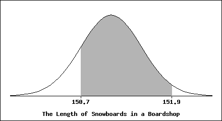
Checkpoint 9.2.10. WebWork - Computing Regular Normal Probabilities.

Length of snowboards in a boardshop are normally distributed with a mean of 151.1 cm and a standard deviation of 0.4 cm. The figure below shows the distribution of the length of snowboards in a boardshop. Calculate the shaded area under the curve. Express your answer in decimal form with at least two decimal place accuracy.

Answer:

Answer.

0.8185948

🔗

In the standard normal distribution, we have considered the case where you get the probability when given an interval. However, what about the reverse problem of finding an interval that would result in a given probability? That is, to solve for example the problem

Φ (b) - Φ (a) = P (a < z < b) = 0.6217 .

🔗

To deal with this we need an "inverse function"

Φ^{- 1} .

Toward that end, consider the simpler problem of solving

Φ (z_{0}) = P (z < z_{0}) = some given probability value = α .

🔗

Then, technically the answer would be

z_{0} = Φ^{- 1} (α) .

🔗

Since integrating the normal probability function is impossible you can expect that finding a nice formula for the inverse of that integration might also be challenging and that is certainly the case. However, you have two options:

🔗
Guessing $z_{0}$ until you get a probabilty that is close enough to $α .$
🔗
Use a calculator that has the inverse built in!

🔗

For most graphing calculators, there is a function called "invNorm" and that is a way to compute values involving

Φ^{- 1} .

Indeed, for example if you wanted to solve

Φ (z_{0}) = P (z < z_{0}) = 0.813

🔗

then just use invNorm(

0.813

) to get

z_{0} \approx - 0.2198 .

🔗


    
        
xxxxxxxxxx
 
1
# Inverse Normal Calculator
2
print("Calculator for Inverse Standard Normal")
3
var("x")
4
@interact(layout=dict(top=[['p0']]))
5
def _(p0=input_box(1/2,width=10,label='probability= ')):
6
    if (p0 > 0.99999999) or (p0 < 0.000032):    # due to the sensitivity of T below
7
        print("Enter a value between 0.000032 and 0.99999999")
8
    else:
9
        T = RealDistribution('gaussian', 1)   # use built-in
10
        z0 = T.cum_distribution_function_inv(p0)  # rel tol 1e-14
11
        pretty_print(html("$$ P(Z < z_0) = \\Phi(z_0) = "+str(p0)+" \\; \\; " +
12
                      "\\Rightarrow \\; \\; z_0 ="+str(z0)+"$$"))
13
        G = plot(T,x,-6,6)+plot(T,x,-4,z0,fill=True,fillcolor='green')
14
        show(G,figsize=(4,2))

    
    
    
    
        
            
                Language:
                
            
        
    
    




    
    
        
        Messages

🔗

Checkpoint 9.2.11. WebWork - Inverse Standard Normal Calculations.

Find the value of the standard normal random variable

z,

called

z_{0}

such that:

(a)

P (z \leq z_{0}) = 0.7699

z_{0} =

(b)

P (- z_{0} \leq z \leq z_{0}) = 0.8568

z_{0} =

(c)

P (- z_{0} \leq z \leq z_{0}) = 0.856

z_{0} =

(d)

P (z \geq z_{0}) = 0.0905

z_{0} =

(e)

P (- z_{0} \leq z \leq 0) = 0.1842

z_{0} =

(f)

P (- 2.26 \leq z \leq z_{0}) = 0.6250

z_{0} =

Answer 1.

0.738518

Answer 2.

1.46398

Answer 3.

1.46106

Answer 4.

1.33768

Answer 5.

0.479476

Answer 6.

0.350185

🔗

While we are at it, can we "go backwards" and figure out the mean and variance if given some probabilities. This requires some problem solving skills and enough provided information to figure things out. For the exercise below, what does it mean to talk about the "middle" percentage of the area? That gives one the mean and also describes a probability of the sort

P (μ - z_{0} σ < X < μ + z_{0} σ),

🔗

where

z_{0}

is a z-value obtained by using the inverse normal distribution function. It might help to draw a picture first of the area under the normal curve described in any such exercise.

🔗

Checkpoint 9.2.12. WebWork - Computing Regular Normal Probabilities.

Consider a normal distribution curve where the middle 65 % of the area under the curve lies above the interval ( 6 , 13 ). Use this information to find the mean,

μ

, and the standard deviation,

σ

, of the distribution.

μ =

σ =

Answer 1.

9.5

Answer 2.

3.74496

🔗

Checkpoint 9.2.13. WebWork - Applying Normal Probabilities.

The physical fitness of an athlete is often measured by how much oxygen the athlete takes in (which is recorded in milliliters per kilogram, ml/kg). The mean maximum oxygen uptake for elite athletes has been found to be

75

with a standard deviation of

5.8 .

Assume that the distribution is approximately normal.

(a)

What is the probability that an elite athlete has a maximum oxygen uptake of at least

70

ml/kg?

answer:

(b)

What is the probability that an elite athlete has a maximum oxygen uptake of

55

ml/kg or lower?

answer:

(c)

Consider someone with a maximum oxygen uptake of

27

ml/kg. Is it likely that this person is an elite athlete? Write "YES" or "NO."

answer:

Answer 1.

0.805675

Answer 2.

0.000282000000000004

Answer 3.

Essentials of Mathematical Probability and Statistics

Search Results:

Section 9.2 The Normal Distribution

Definition 9.2.1. The Normal Distribution.

Theorem 9.2.2. Standard Normal Distribution.

Proof.

Checkpoint 9.2.3. WebWork - Computing Standard Normal Probabilities.

Checkpoint 9.2.4. WeBWorK - Computing Normal Probabilities when non-Standard.

Theorem 9.2.5. Verifying the normal probability function.

Proof.

Theorem 9.2.6. Verifying the normal probability mean.

Proof.

Theorem 9.2.7. Verifying the normal probability variance.

Proof.

Theorem 9.2.8. Normal Distribution Maximum.

Proof.

Theorem 9.2.9. Normal Distribution Points of Inflection.

Proof.

Checkpoint 9.2.10. WebWork - Computing Regular Normal Probabilities.

Checkpoint 9.2.11. WebWork - Inverse Standard Normal Calculations.

Checkpoint 9.2.12. WebWork - Computing Regular Normal Probabilities.

Checkpoint 9.2.13. WebWork - Applying Normal Probabilities.