Expected Value

Section 5.4 Expected Value

Blaise Pascal was a 17th century mathematician and philosopher who was accomplished in many areas but may likely be best known to you for his creation of what is now known as Pascal’s Triangle. As part of his philosophical pursuits, he proposed what is known as "Pascal’s wager". It suggests two mutually exclusive outcomes: that God exists or that he does not. His argument is that a rational person should live as though God exists and seek to believe in God. If God does not actually exist, such a person will have only a finite loss (some pleasures, luxury, etc.), whereas they stand to receive infinite gains as represented by eternity in Heaven and avoid an infinite losses of eternity in Hell. This type of reasoning is part of what is known as "decision theory".

🔗

You may not confront such dire payouts when making your daily decisions but we need a formal method for making these determinations precise. The procedure for doing so is what we call expected value.

🔗

Definition 5.4.1. Expected Value.

🔗

Given a random variable

X

over space

R,

corresponding probability function

f (x)

and "value function"

v (x),

the expected value of

v (x)

is given by

E = E [v (X)] = \sum_{x \in R} v (x) f (x)

🔗

provided

X

is discrete, or

E = E [v (X)] = \int_{R} v (x) f (x) d x

🔗

provided

X

is continuous.

🔗

Theorem 5.4.2. Expected Value is a Linear Operator.

🔗

🔗
$E [c] = c$
🔗
$E [c v (X)] = c E [v (X)]$
🔗
$E [v (X) + w (X)] = E [v (X)] + E [w (X)]$

🔗

Proof.

Each of these follows by utilizing the corresponding linearity properties of the summation and integration operations. For example, to verify part three in the continuous case:

\begin{aligned} E [v (X) + w (X)] & = \int_{x \in R} [v (x) + w (x)] f (x) d x \\ = \int_{x \in R} v (x) f (x) d x + \int_{x \in R} w (x) f (x) d x \\ = E [v (X)] + E [w (X)] . \end{aligned}

🔗

Example 5.4.3. Discrete Expected Value.

Consider

f (x) = x / 10

over

R

= {1,2,3,4} where the payout is 10 euros if x=1, 5 euros if x=2, 2 euros if x=3 and -7 euros if x = 4. Then your value function would be

v (1) = 10, v (2) = 5, v (3) = 2, v (4) = - 7.

Computing the expect payout gives

E = 10 \times 1 / 10 + 5 \times 2 / 10 + 2 \times 3 / 10 - 7 \times 4 / 10 = - 2 / 10

Therefore, the expected payout is actually negative due to a relatively large negative payout associated with the largest likelihood outcome and the larger positive payout only associated with the least likely outcome.

🔗

Example 5.4.4. Continuous Expected Value.

Consider

f (x) = x^{2} / 3

over

R

= [-1,2] with value function given by

v (x) = e^{x} - 1 .

Then, the expected value for

v (x)

is given by

E = \int_{- 1}^{2} (e^{x} - 1) \cdot x^{2} / 3 = - 1 / 9 \cdot (e + 15) \cdot e^{- 1} + 2 / 3 \cdot e^{2} - 8 / 9 \approx 3.3129

🔗

Definition 5.4.5. Theoretical Measures.

🔗

Given a random variable with probability function f(x) over space R

🔗
The mean of $X = μ = E [x]$
🔗
The variance of $X = σ^{2} =$ Var(X) $= E [(x - μ)^{2}]$
🔗
The skewness of $X = γ_{1} = \frac{E [(x - μ)^{3}]}{σ^{3}}$
🔗
The kurtosis of $X = γ_{2} = \frac{E [(x - μ)^{4}]}{σ^{4}}$

🔗

Theorem 5.4.6. Alternate Formulas for Theoretical Measures.

🔗

🔗
$σ^{2} = E [x^{2}] - μ^{2} = E [X (x - 1)] + μ - μ^{2}$
🔗
$γ_{1} = \frac{1}{σ^{3}} \cdot [E [X^{3}] - 3 μ E [X^{2}] + 2 μ^{3}]$
🔗
$γ_{2} = \frac{1}{σ^{4}} \cdot [E [X^{4}] - 4 μ E [X^{3}] + 6 μ^{2} E [X^{2}] - 3 μ^{4}]$

🔗

Proof.

In each case, expand the binomial inside and use the linearity of expected value.

🔗

Checkpoint 5.4.7. WebWork - Expected Value.

E [X] = 4

and

Var (X) = 1,

then

E [(4 + 5 X)^{2}] =

and

Var (3 + 5 X) =

Answer 1.

601

Answer 2.

25

🔗

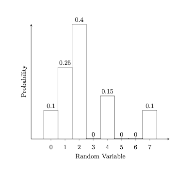
Consider the following example when computing these statistics for a discrete variable. In this case, we will utilize a variable with a relatively small space so that the summations can be easily done by hand. Indeed, consider

Table 5.4.8. Discrete Probability Function Example

X	f(x)
0	0.10
1	0.25
2	0.40
4	0.15
7	0.10

🔗

Using the definition of mean 1 as a sum,

\begin{aligned} μ & = 0 \cdot 0.10 + 1 \cdot 0.25 + 2 \cdot 0.40 + 4 \cdot 0.15 + 7 \cdot 0.10 \\ = 0 + 0.25 + 0.80 + 0.60 + 0.70 \\ = 2.35 \end{aligned}

🔗

Notice where this lies on the probability histogram for this distribution.

🔗

For the variance 2 and using the alternate formulation 1

\begin{aligned} σ^{2} & = E [X^{2}] - μ^{2} \\ = [0^{2} \cdot 0.10 + 1^{2} \cdot 0.25 + 2^{2} \cdot 0.40 + 4^{2} \cdot 0.15 + 7^{2} \cdot 0.10] - {2.35}^{2} \\ = 0 + 0.25 + 1.60 + 2.40 + 4.90 - 5.5225 \\ = 9.15 - 5.225 \\ = 3.6275 \end{aligned}

🔗

and so the standard deviation

σ = \sqrt{3.6275} \approx 1.90 .

Notice that 4 times this value encompasses almost all of the range of the distribution.

🔗

For the skewness 3 and using the alternate formulation 2

\begin{aligned} Numerator = & E [X^{3}] - 3 μ E [X^{2}] + 2 μ^{3} \\ = [0^{3} \cdot 0.10 + 1^{3} \cdot 0.25 + 2^{3} \cdot 0.40 + 4^{3} \cdot 0.15 + 7^{3} \cdot 0.10] - 3 \cdot 2.35 \cdot 9.15 + 2 \cdot {2.35}^{3} \\ \approx 0 + 0.25 + 3.20 + 9.60 + 34.3 - 64.5075 + 25.96 \\ = 47.35 - 64.5075 + 25.96 \\ \approx 8.80 \end{aligned}

🔗

which yields a skewness of

γ_{1} = 8.80 / σ^{3} \approx 1.27 .

This indicates a slight skewness to the right of the mean. You can notice the 4 and 7 entries on the histogram illustrate a slight trailing off to the right.

🔗

Finally, for kurtosis 4 and using the alternate formulation 3

\begin{aligned} Numerator = & E [X^{4}] - 4 μ E [X^{3}] + 6 μ^{2} E [X^{2}] - 3 μ^{4} \\ = [0^{4} \cdot 0.10 + 1^{4} \cdot 0.25 + 2^{4} \cdot 0.40 + 4^{4} \cdot 0.15 + 7^{4} \cdot 0.10] - 4 \cdot 2.35 \cdot 47.35 + 6 \cdot {2.35}^{2} \cdot {9.15}^{2} - 3 \cdot {2.35}^{4} \\ \approx 0 + 0.25 + 6.40 + 38.4 + 240.1 - 445.09 + 303.19 - 91.49 \\ \approx 285.15 - 445.09 + 303.19 - 91.49 \\ \approx 51.75 \end{aligned}

🔗

which yields a kurtosis of

γ_{2} = 51.75 / σ^{4} \approx 3.93

which also notes that the data appears to have a modestly bell-shaped distribution.

🔗

Checkpoint 5.4.9. WebWork - Random Variables.

Find the expected value for the random variable:

$X$	3	5	6	8
$P (X)$	0.21	0.16	0.25	0.38

E (X) =

Answer.

5.97

🔗

Checkpoint 5.4.10. WebWork - More Random Variables.

Prizes and the chances of winning in a sweepstakes are given in the table below.

Prize	Chances
$10,000,000	1 chance in 300,000,000
$350,000	1 chance in 150,000,000
$50,000	1 chance in 80,000,000
$20,000	1 chance in 5,000,000
$500	1 chance in 800,000
A watch valued at $60	1 chance in 7,000

(a)

Find the expected value (in dollars) of the amount won by one entry.

(b)

Find the expected value (in dollars) if the cost of entering this sweepstakes is the cost of a postage stamp (34 cents)

Answer 1.

0.0494880952380952

Answer 2.

- 0.290511904761905

Solution.

W

be the amount of money (in dollars) won by an entry. Then

\begin{aligned} E [W] = & 10000000 \cdot P (W = 10000000) + 350000 \cdot P (W = 350000) + 50000 \cdot P (W = 50000) \\ + 20000 \cdot P (W = 20000) + 500 \cdot P (W = 500) + 60 \cdot P (W = 60) \\ = \frac{10000000}{300000000} + \frac{350000}{150000000} + \frac{50000}{80000000} + \frac{20000}{5000000} + \frac{500}{800000} + \frac{60}{7000} \\ = 0.0494880952380952 \end{aligned}

So the expected value of the amount won by one entry in the sweepstakes is about 5 cents. (b) Let

X

be the net earnings from one entry into the sweepstakes. Then

X = W - 0.34,

E [X] = E [W - 0.34] = E [W] - 0.34 = - 0.290511904761905 .

Hence, taking into account the cost of postage, there is an expected loss of about 29 cents from one entry into the sweepstakes.

🔗

Checkpoint 5.4.11. WebWork - Even More.

The table below summarizes the number of surface flaws found on the paintwork of new cars following their inspection after primer paint was applied by a new method:

No. of flaws	No. of cars
0	3
1	7
2	12
3	11
4	3
5	2
6	2

Part a) Find the mean number of flaws per car. Please give your answer to two decimal places.

The mean number of flaws per car is:

Part b)

Find the variance of the number of flaws per car. Please give your answer to two decimal places.

The variance of the number of flaws per car is:

Answer 1.

2.45

Answer 2.

2.151

Solution.

Here

n = 40

and the sample mean is

\bar{x} = \frac{3 \times 0 + 7 \times 1 + 12 \times 2 + 11 \times 3 + 3 \times 4 + 2 \times 5 + 2 \times 6}{40} = 2.45 .

The sample variance is

\frac{3 {(0 - 2.45)}^{2} + 7 {(1 - 2.45)}^{2} + 12 {(2 - 2.45)}^{2} + 11 {(3 - 2.45)}^{2} + 3 {(4 - 2.45)}^{2} + 2 {(5 - 2.45)}^{2} + 2 {(6 - 2.45)}^{2}}{39}

which is 2.151.

🔗

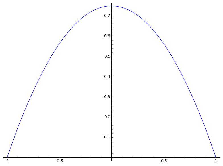
Consider the following example when computing these statistics for a continuous variable. Let

f (x) = \frac{3}{4} \cdot (1 - x^{2})

over

R = [- 1, 1] .

🔗

Then for the mean 1

\begin{aligned} μ & = \int_{- 1}^{1} x \cdot \frac{3}{4} \cdot (1 - x^{2}) d x \\ = \int_{- 1}^{1} \frac{3}{4} \cdot (x - x^{3}) d x \\ = \frac{3}{4} \cdot (x^{2} / 2 - x^{4} / 4) |_{- 1}^{1} \\ = \frac{3}{4} \cdot [(1 / 2) - (1 / 4)] - [(1 / 2) - (1 / 4)] \\ = 0 \end{aligned}

🔗

as expected since the probability function is symmetric about x=0.

🔗

For the variance 5.4.6

\begin{aligned} σ^{2} & = \int_{- 1}^{1} x^{2} \cdot \frac{3}{4} \cdot (1 - x^{2}) d x - μ^{2} \\ = \int_{- 1}^{1} \cdot \frac{3}{4} \cdot (x^{2} - x^{4}) d x - 0 \\ = \frac{3}{4} \cdot (x^{3} / 3 - x^{5} / 5) |_{- 1}^{1} \\ = \frac{3}{4} \cdot 2 \cdot (1 / 3 - 1 / 5) \\ = \frac{3}{4} \cdot \frac{4}{15} \\ = \frac{1}{5} \end{aligned}

🔗

and taking the square root gives a standard deviation slightly less than 1/2. Notice that four times this value encompasses almost all of the range of the distribution.

🔗

For the skewness 3, notice that the graph is symmetrical about the mean and so we would expect a skewness of 0. Just to check it out

\begin{aligned} Numerator = & E [X^{3}] - 3 μ E [X^{2}] + 2 μ^{3} \\ = \int_{- 1}^{1} x^{3} \cdot \frac{3}{4} \cdot (1 - x^{2}) d x - 3 E [X^{2}] \cdot 0 + 0^{3} \\ = \int_{- 1}^{1} \cdot \frac{3}{4} \cdot (x^{3} - x^{5}) d x \\ = \frac{3}{4} \cdot (x^{4} / 4 - x^{6} / 6) |_{- 1}^{1} \\ = 0 \end{aligned}

🔗

as expected without having to actually complete the calculation by dividing by the cube of the standard deviation.

🔗

Finally, note that the probability function in this case is modestly close to a bell shaped curve so we would expect a kurtosis 4 and using the alternate formulation 4 in the vicinity of 3. Indeed, noting that (conveniently)

μ = 0

gives

\begin{aligned} Numerator = & E [X^{4}] - 4 μ E [X^{3}] + 6 μ^{2} E [X^{2}] - 3 μ^{4} \\ = \int_{- 1}^{1} x^{4} \cdot \frac{3}{4} \cdot (1 - x^{2}) d x \\ = \frac{3}{4} \cdot (x^{5} / 5 - x^{7} / 7) |_{- 1}^{1} \\ = \frac{3}{4} \cdot 2 (1 / 5 - 1 / 7) \\ = \frac{3}{35} \end{aligned}

🔗

and so by dividing by

σ^{4} = {\sqrt{\frac{1}{5}}}^{4} = \frac{1}{25}

gives a kurtosis of

γ_{2} = \frac{3}{35} / \frac{1}{25} = \frac{75}{35} \approx 2.14 .

🔗

Example 5.4.12.

Consider our previous example 5.4.4. To compute the mean 1 and variance 2 (and hence the standard deviation) for this distribution,

μ = \int_{- 1}^{2} x \cdot x^{2} / 3 d x = \int_{- 1}^{2} x^{3} / 3 d x = \frac{2^{4}}{12} - \frac{(- 1)^{4}}{12} = \frac{15}{12} = \frac{5}{4}

and by using the alternate formulas 5.4.6

\begin{aligned} σ^{2} & = E [X^{2}] - μ^{2} \\ = \int_{- 1}^{2} x^{2} \cdot x^{2} / 3 d x - μ^{2} \\ = \int_{- 1}^{2} x^{4} / 3 d x - {(\frac{5}{4})}^{2} \\ = \frac{2^{5}}{15} - \frac{(- 1)^{5}}{15} - \frac{25}{16} \\ = \frac{33}{15} - \frac{25}{16} = \frac{51}{80} \end{aligned}

which gives

σ = \sqrt{\frac{51}{80}} \approx 0.7984 .

For skewness 3, note that in computing the variance above you also found that

E [X^{2}] = \frac{11}{5} .

So, once again by using the alternate formulas 5.4.6

E [X^{3}] = \int_{- 1}^{2} x^{3} \cdot x^{2} / 3 d x = \frac{x^{6}}{18} |_{- 1}^{2} = \frac{7}{2}

and so

γ_{1} = \frac{\frac{7}{2} - 3 \cdot \frac{5}{4} \cdot \frac{11}{5} + 2 \cdot (\frac{5}{4})^{3}}{{\sqrt{\frac{51}{80}}}^{3}}

For kurtosis 4, you can reuse

E [X^{3}] = \frac{7}{2}

and

E [X^{2}] = \frac{11}{5}

and the alternate formulas 5.4.6 to determine

E [(X - μ)^{4}] = E [X^{4}] - 4 μ \cdot E [X^{3}] + 6 μ^{2} \cdot E [X^{2}] - 3 μ^{4}

which is the numerator for the kurtosis.

🔗

Example 5.4.13. Roulette.

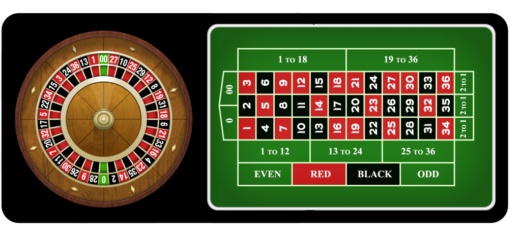
Roulette is a gambling game popular in may casinos in which a player attempts to win money from the casino by predicting the location that a ball lands on in a spinning wheel. There are two variations of this game...the American version and the European version. The difference being that the American version has one additional numbered slot on the wheel. The American version of the game will be used for the purposes of this example.

A Roulette wheel consists of 38 equally-sized sectors identified with the numbers 1 through 36 plus 0 and 00. The 0 and 00 sectors are colored green and half of the remaining numbers are in sectors colored red with the remainder colored black. A steel ball is dropped onto a spinning wheel and as the wheel comes to rest the sector in which it comes to rest is noted. It is easy to determine that the probability of landing on any one of the 38 sectors is 1/38. A picture of a typical American-style wheel and betting board is given by

. (Found at BigFishGames.com.)

Since this is a game in a casino, there must be the opportunity to bet (and likely lose) money. For the remainder of this example we will assume that you are betting 1 dollar each time. If you were to bet more then the values would scale correspondingly. However, if you place your bet on any single number and the ball ends up on the sector corresponding to that number, you win a net of 35 dollars. If the ball lands elsewhere you lose your dollar. Therefore the expected value of winning if you bet on one number is

E [win on one] = 35 \cdot \frac{1}{38} - 1 \cdot \frac{37}{38} = - \frac{2}{38}

which is a little more than a nickel loss on average.

You can bet on two numbers as well and if the ball lands on either of the two then you win a payout in this case of 17 dollars. Therefore the expected value of winning if you bet on two numbers is

E [win on two numbers] = 17 \cdot \frac{2}{38} - 1 \cdot \frac{36}{38} = - \frac{2}{38} .

Continuing, you can bet on three numbers and if the ball lands on any of the three then you win a payout of 11 dollars. Therefore the expected value of winning if you bet on three numbers is

E [win on three numbers] = 11 \cdot \frac{3}{38} - 1 \cdot \frac{35}{38} = - \frac{2}{38} .

You can bet on all reds, all blacks, all evens (ignoring 0 and 00), or all odds and get your dollar back. The expected value for any of these options is

E [win on eighteen numbers] = 1 \cdot \frac{18}{38} - 1 \cdot \frac{20}{38} = - \frac{2}{38} .

There is one special way to bet which uses the the 5 numbers {0, 00, 1, 2, 3} and pays 6 dollars. This is called the "top line of basket". Notice that the use of five numbers will make getting the same expected value as the other cases impossible using regular dollars and cents. The expected value of winning in this case us

E [win on top line of basket] = 6 \cdot \frac{5}{38} - 1 \cdot \frac{33}{38} = - \frac{3}{38}

which is of course worse and is the only normal way to bet on roulette which has a different expected value.

There are other possible ways to bet on roulette but none provide a better expected value of winning. The moral of this story is that you should never bet on the 5 number option and if you ever get ahead by winning on roulette using any of the possible options then you should probably stop quickly since over a long period of time it is expected that you will lose an average of

\frac{1}{19}

dollars per game.

🔗

Going back to Pascal’s wager, let

🔗
X = 0 represent disbelief when a benevolent God doesn’t exist
🔗
X = 1 represent disbelief when a benevolent God does exist
🔗
Y = 2 represent belief when a benevolent God does exist
🔗
Y = 3 represent belief when a benevolent God does not exist

🔗

Presume that p is the likelihood that a benevolent God exists. Then you can compute the expected value of disbelief and the expect value of belief by first creating a value function. Below, for argument sake we are somewhat randomly assign a value of one million to disbelief if a benevolent God doesn’t exist. The conclusions are the same if you choose any other finite number...

\begin{matrix} v (0) = 1, 000, 000, f (0) = 1 - p \\ v (1) = - \infty, f (1) = p \\ v (2) = \infty, f (2) = p \\ v (3) = 0, f (3) = 1 - p \end{matrix}

🔗

Then, looking at the disbelief random variable X with a probability function

f (0) = 1 - p, f (1) = p,

\begin{aligned} E [disbelief] & = v (0) f (0) + v (1) f (1) \\ = 1000000 \times (1 - p) - \infty \times p \\ = - \infty \end{aligned}

🔗

if p>0. On the other hand, looking at the belief random variable Y with probability function

g (2) = p, g (3) = 1 - p,

\begin{aligned} E [belief] & = v (2) g (2) + v (3) g (3) \\ = \infty \times p + 0 \times (1 - p) \\ = \infty \end{aligned}

🔗

if p>0. So Pascal’s conclusion is that if there is even the slightest chance that a benevolent God exists then belief is the smart and scientific choice.

Essentials of Mathematical Probability and Statistics

Search Results:

Section 5.4 Expected Value

Definition 5.4.1. Expected Value.

Theorem 5.4.2. Expected Value is a Linear Operator.

Proof.

Example 5.4.3. Discrete Expected Value.

Example 5.4.4. Continuous Expected Value.

Definition 5.4.5. Theoretical Measures.

Theorem 5.4.6. Alternate Formulas for Theoretical Measures.

Proof.

Checkpoint 5.4.7. WebWork - Expected Value.

Checkpoint 5.4.9. WebWork - Random Variables.

Checkpoint 5.4.10. WebWork - More Random Variables.

Checkpoint 5.4.11. WebWork - Even More.

Example 5.4.12.

Example 5.4.13. Roulette.