Section 1.5 Statistical Measures of Variation
Consider the data from the class collected in the previous section regarding how far each person has to commute to get to class each day. Consider whether the commute distance is about the same for each person or whether those distances vary widely. What would change about your answer if you changed the units from (say) miles to kilometers or meters or inches or nanometers?
These measures provide some indication of how much the data set is "spread out". Indeed, note that the data sets {-2,-1,0,1,2} and {-200,-100,0,100,200} have the same mean but one is much more spread out than the other. Measures of variation should catch this difference.
Definition 1.5.2. Range:.
Using the order statistics,
\begin{equation*}
y_n - y_1.
\end{equation*}
It is trivial to note that the range is very easy to compute but it completely ignores all data values except for the two ends.
From the Presidential data 1.3.2, the maximum is 69 and the minimum is 46 so the range is 23, the difference of these two.
Definition 1.5.3. Interquartile Range (IQR):.
\begin{equation*}
IQR = P^{0.75} - P^{0.25} = Q_3 - Q_1.
\end{equation*}
For the data set {2, 5, 8, 10}, you have found that \(Q_1 = 2.75\) and \(Q_3 = 9.5\) when using the "n+1" method (and slightly different if using the "n-1" method.) Therefore,
\begin{equation*}
IQR = 9.5 - 2.75 = 6.75.
\end{equation*}
Let’s now consider a measure of variation that is the counterpart to the mean in that it involves a computation that utilizes the actual values of all the data.
Average Deviation from the Mean (Population): Given a population data set \(x_1, x_2, ... , x_n\) with mean \(\mu\) each term deviates from the mean by the value \(x_k - \mu\text{.}\) So, averaging these gives
\begin{equation*}
\frac{\sum_{k=1}^n (x_k-\mu)}{n} = \frac{\sum_{k=1}^n x_k}{n} - \frac{\sum_{k=1}^n \mu}{n} = \mu - \mu = 0.
\end{equation*}
This metric is therefore always zero for any provided set of data since cancellation makes this not useful. You should have expected this to be true since the definition of the mean is indeed the place where the data is "balanced". So, we need to determine ways to avoid cancellation.
Average Absolute Deviation from the Mean (Population):
\begin{equation*}
\frac{\sum_{k=1}^n \left | x_k-\mu \right |}{n}
\end{equation*}
which, although nicely stated, is difficult to deal with algebraically since the absolute values do not simplify well algebraically. Indeed, it is easy to see that, for example when n=3, the mean lies somewhere between \(y_1\) and \(y_3\) (using the ordered data) but could be on either side of \(y_2\) and so
\begin{equation*}
|y_1-\mu| + |y_2 - \mu| + |y_3 - \mu| = -(y_1-\mu) + ?(y_2 - \mu) + |y_3 - \mu|
\end{equation*}
where the ? is either a + or a - but it could be either in general. To avoid this algebraic roadblock, we can look for another way to nearly accomplish the same goal by squaring and then square rooting.
Average Squared Deviation from the Mean (Population):
\begin{equation*}
\frac{\sum_{k=1}^n ( x_k-\mu )^2}{n}
\end{equation*}
which will always be non-negative but can be easily expanded using algebra. Since this is a mouthful, this measure is generally called the "variance".
Using the average squared deviation from the mean, differences have been squared. Thus all of the squared differences added are non-negative but very small ones have been made even smaller and larger ones have been made relatively larger. To undo this scaling issue, one must take a square root to get things back into the right ball park.
Definition 1.5.4. Variance and Standard Deviation.
The variance is the average squared deviation from the mean. If this data comes from the entire universe of possibilities then we call it a population variance and denote this value by \(\sigma^2\text{.}\) Therefore
\begin{equation*}
\sigma^2 = \frac{\sum_{k=1}^n ( x_k-\mu )^2}{n}
\end{equation*}
The standard deviation is the square root of the variance. If this data comes from the entire universe of possibilities then we call it a population standard deviation and denote this value by \(\sigma\text{.}\) Therefore
\begin{equation*}
\sigma = \sqrt{\frac{\sum_{k=1}^n ( x_k-\mu )^2}{n}}.
\end{equation*}
If data comes from a sample of the population then we call it a sample variance and denote this value by
\begin{equation*}
v = \frac{\sum_{k=1}^n ( x_k-\overline{x} )^2}{n}.
\end{equation*}
Sample data tends to reflect certain "biases". For example, a small data set is unlikely to contain a member of the data set that is far away from the major portion of the data. However, data values that are far from the mean provide a much greater contribution to the calculation of v than do values that are close to the mean. Technically, bias is defined mathematically using something called "expected value" and would be discussed in a course that might follow this one.
To account for this, we increase the value computed for v slightly by \(\frac{n}{n-1}\) to give the sample variance via
\begin{equation*}
s^2 = \frac{n}{n-1} v = \frac{n}{n-1}\frac{\sum_{k=1}^n ( x_k-\overline{x} )^2}{n} = \frac{\sum_{k=1}^n ( x_k-\overline{x} )^2}{n-1}.
\end{equation*}
and the sample standard deviation \(s\) similarly as the square root of the sample variance.
From the data {2,5,8,10}, you have found that the mean is 6.25. Computing the variance then involves accumulating and averaging the squared differences of each data value and this mean. Then
\begin{align*}
& \frac{1}{4} \left ( (2-6.25)^2 + (5-6.25)^2 + (8-6.25)^2 + (10-6.25)^2 \right ) \\
& = \frac{18.0625 + 1.5625 + 3.0625 + 14.0625}{4} \\
& = \frac{36.75}{4}\\
& = 9.1875.
\end{align*}
Theorem 1.5.5. Alternate Forms for Variance.
\begin{align*}
\sigma^2 & = \left ( \frac{\sum_{k=1}^n x_k^2 }{n} \right ) - \mu^2 \\
& = \left [ \frac{\sum_{k=1}^n x_k(x_k - 1)}{n} \right ] + \mu - \mu^2
\end{align*}
Proof.
\begin{align*}
\sigma^2 & = \frac{\sum_{k=1}^n ( x_k-\mu )^2}{n}\\
& = \frac{\sum_{k=1}^n ( x_k^2 - 2x_k \mu + \mu^2 )}{n}\\
& = \frac{\sum_{k=1}^n x_k^2 - 2\mu \sum_{k=1}^n x_k + n \mu^2 )}{n}\\
& = \left ( \frac{\sum_{k=1}^n x_k^2 }{n} \right ) - \mu^2
\end{align*}
The second part is proved similarly. Using the first part of the proof above,
\begin{align*}
\sigma^2 & = \frac{\sum_{k=1}^n ( x_k-\mu )^2}{n}\\
& = \left ( \frac{\sum_{k=1}^n x_k^2 }{n} \right ) - \mu^2\\
& = \left ( \frac{\sum_{k=1}^n x_k (x_k - 1) + x_k }{n} \right ) - \mu^2\\
& = \left ( \frac{\sum_{k=1}^n x_k (x_k - 1)}{n} \right ) + \mu - \mu^2
\end{align*}
Example 1.5.6. Computing means and variances by hand.
In the data table below, notice that the \(x_k\) column would be the given data values but the column for \(x_k^2\) you could easily compute. Table 1.5.7. Sample Grouped Data
So, \(\Sigma x_k = 9\) and \(\Sigma x_k^2 = 35\text{.}\) Therefore \(\overline{x} = \frac{9}{6} = \frac{3}{2}\) and \(v = \frac{\Sigma x_k^2}{6} - (\overline{x})^2 = \frac{35}{6} - (\frac{3}{2})^2 = \frac{70-18}{12} = \frac{26}{6}\text{.}\)
| \(x_k\) | \(x_k^2\) |
| 1 | 1 |
| -1 | 1 |
| 0 | 0 |
| 2 | 4 |
| 2 | 4 |
| 5 | 25 |
Therefore, \(s^2 = \frac{6}{5} \times v = \frac{26}{5}\text{.}\)
Checkpoint 1.5.8. Computing Descriptive Statistics.
The times (in seconds) between fifteen consecutive eruptions of a geyser were as follows:
878, 871, 906, 933, 930, 852, 890, 861, 882, 888, 897, 899, 879, 888, 848
By entering the data into R, find the following (giving answers to two decimal places):
Part a) The sample mean is (\({\rm sec}\)).
Part b) The sample variance is (\({\rm sec}^{2}\)).
Part c) The sample median is (\({\rm sec}\)).
Part d) The sample IQR is (\({\rm sec}\)).
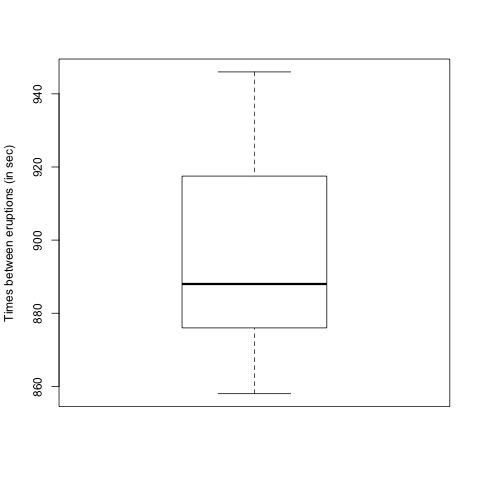
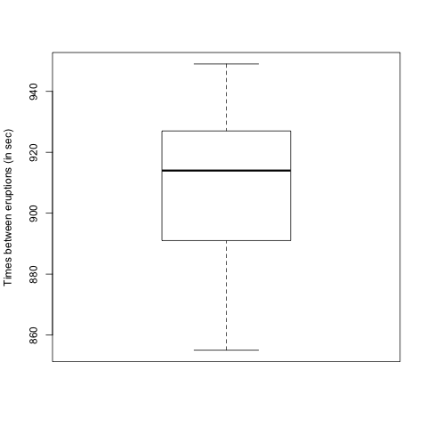
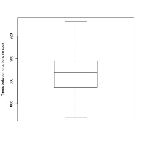
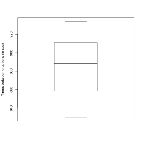
Part e) Which of the following is a boxplot of the data?
- A
- B
- C
- D
 |
 |
| A | B |
 |
 |
| C | D |
(Click on a graph to enlarge it.)
Answer 1.
Answer 2.
Answer 3.
Answer 4.
Answer 5.
Solution.
\(886.8\)
\(602.029\)
\(888\)
\(23.5\)
\(\text{C}\)
Suppose you have entered the data in R as follows:
\(\verb| x \lt - c( 878, 871, 906, 933, 930, 852, 890, 861, 882, 888, 897, 899, 879, 888, 848 ) |\)
Then the sample mean, sample variance, sample median, and sample IQR are obtained as follows:
\(\verb|mean(x) |\)
\(\verb|var(x) |\)
\(\verb|median(x) |\)
\(\verb|IQR(x) |\)
You can obtain a boxplot by typing
\(\verb|boxplot( x, ylab = "Times between eruptions (in sec)", id.method="y") |\)
For the data as given, the sample mean is 886.8 sec, the variance is 602.029 min\({}^{2}\text{,}\) the median is 888 min and the IQR is 23.5 min (from R’s default type; it may be quite different if you used a different type.)
Once again, we can compute these descriptive statistics using R. We again display a box and whisker diagram and you should now notice the the "box" corresponds to the IQR.
Experiment in the above interactive cell by using one of the built-in data sets.
We can also consider once again the Population of the individual USA states according to the 2013 Census is considered below.
Checkpoint 1.5.9. USA State Population Measures of Variation.
Using the US Census Bureau state populations 1.4.9 (in millions) for 2014 provided earlier, determine the range, quartiles, and variance for this sample data.
Solution.Again, you should note that these are already in order so the range is quickly found to be
\begin{equation*}
y_n - y_1 = 38.3 - 0.6 = 37.7
\end{equation*}
million residents.
For IQR, we first must determine the quartiles. The median (found earlier) already is the second quartile so we have \(Q_2 = 4.5\) million. For the other two, the formula for computing percentiles gives you the 25th percentiile
\begin{gather*}
(n+1)p = 51(1/4) = 12.75\\
Q_1 = P^{0.25} = 0.25 \times 1.9 + 0.75 \times 2.1 = 2.05
\end{gather*}
and the 75th percentile
\begin{gather*}
(n+1)p = 51(3/4) = 38.25\\
Q_3 = P^{0.75} = 0.75 \times 7 + 0.25 \times 8.3 = 7.325.
\end{gather*}
Hence, the IQR = 7.325 - 2.05 = 5.275 million residents.
From the computation before, again note that n=51 since the District of Columbia is included. The mean of this data found before was found to be approximately 6.20 million residents. So, to determine the variance you may find it easier to compute using the the alternate variance formulas 1.5.5.
\begin{align*}
v & = \left ( \frac{\sum_{k=1}^n y_k^2 }{n} \right ) - \mu^2\\
& \approx \frac{4434.37}{51} - (6.20)^2\\
& = 48.51
\end{align*}
and so you get a sample variance of
\begin{equation*}
s^2 \approx \frac{51}{50} \cdot 48.51 = 49.48
\end{equation*}
and a sample standard deviation of
\begin{equation*}
s \approx \sqrt{49.48} \approx 7.03
\end{equation*}
million residents.
The interquartile range is sometimes also called the interquantile range. It must be noted that R computes the IQR differently for some reason. You can look up the R documentation to see what they do but notice that you can force R to use the standard approach as well. Below, for example, the interactive cell determine the IQR using R’s preferred method. However, to use the method from this text, you can make the function call IQR(data, type=2). This might be helpful to know when working on some WeBWorK exercises where the author could be using R to compute the correct answer.
The state population data set has been entered for you in the R cell below...
