Section 6.4 Hypergeometric Distribution
For the discrete uniform distribution, the presumption is that you will be making a selection one time from the collection of items. However, if you want to take a larger sample without replacement from a distribution in which originally all are equally likely then you will end up with something which will not be uniform.
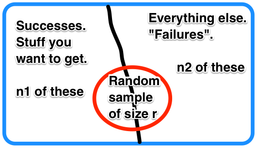
Indeed, consider a collection of n items from which you want to take a sample of size r without replacement. If \(n_1\) of the items are "desired" and the remaining \(n_2 = n - n_1\) are not, let the random variable X measure the number of items from the first group in your sample with \(R = \{0, 1, ..., min {r,n_1} \}\text{.}\) The resulting collection of probabilities is called a Hypergeometric Distribution.
For a Hypergeometric random variable with \(R\) = {0, 1, ..., r} and assuming \(n_1 \ge r\) and \(n-n_1 \ge r\text{,}\)
Theorem 6.4.1. Hypergeometric Probability Function.
Proof.
For the following, we will presume thatSince you are sampling without replacement and trying only measure the number of items from your desired group in the sample, then the space of X will include R = {0, 1, ..., r} assuming \(n_1 \ge r\) and \(n-n_1 \ge r\text{.}\) In the case when r is too large for either of these, the formulas below will follow noting that binomial coefficients are zero if the top is smaller than the bottom or if the bottom is negative.
So f(x) = P(X = x) = P(x from the sample are from the target group and the remainder are not). Breaking these up gives
For example, suppose that you have a bag of assorted candies but you really prefer the little dark chocolate bars. Because you are obsessive, you first empty the whole bag onto your desk and discover that the bag contains 33 equally-sized candy bars of which 6 of them are your delightful dark chocolate bars. Putting the bars randomly back into the bag, you find that a friend's friend's friend walks into the room and grabs a handful of 5 candy bars from your bag. You are shocked and would like to know the probability that this person got 2 or more of your dark chocolate candy bars.
As a good prob/stats student you recognize that this situation fits the requirements of the hypergeometric distribution with \(n_1 = 6, n_2 = 27, r=5\) and you want \(P(X \ge 2)\text{.}\) You determine that it would be easier to compute the complement
Therefore,
or after some simplification
Therefore, you have about 1 chance out of 5 that the friend got 2 or more of your bars. You can be somewhat confident that plenty of dark chocolate bars remain hoarded for yourself.
Theorem 6.4.2. Properties of the Hypergeometric Distribution.
- \(f(x) = \frac{\binom{n_1}{x} \binom{n-n_1}{r-x}}{\binom{n}{r}}\) satisfies the properties of a probability function.
- \(\displaystyle \mu = r \frac{n_1}{n}\)
- \(\displaystyle \sigma^2 = r \frac{n_1}{n} \frac{n_2}{n} \frac{n-r}{n-1}\)
- \(\displaystyle \gamma_1 = \frac{(n - 2 n_1)\sqrt{n-1}(n - 2r)}{r n_1 (n - n_1) \sqrt{n-r}(n-2)}\)
- \(\gamma_2 = \) very complicated!
Proof.
-
\begin{align*} \sum_{x=0}^n \binom{n}{x} y^x & = (1+y)^n, \text{ by the Binomial Theorem}\\ & = (1+y)^{n_1} \cdot (1+y)^{n_2} \\ & = \sum_{x=0}^{n_1} \binom{n_1}{x} y^x \cdot \sum_{x=0}^{n_2} \binom{n_2}{x} y^x \\ & = \sum_{x=0}^n \sum_{t=0}^r \binom{n_1}{r} \binom{n_2}{r-t} y^x \end{align*}
Equating like coefficients for the various powers of y gives
\begin{equation*} \binom{n}{r} = \sum_{t=0}^r \binom{n_1}{r} \binom{n_2}{r-t}. \end{equation*}Dividing gives
\begin{equation*} 1 = \sum_{x=0}^r f(x). \end{equation*} -
For the mean
\begin{align*} \sum_{x=0}^n x \frac{\binom{n_1}{x} \binom{n-n_1}{r-x}}{\binom{n}{r}} & = \frac{1}{\binom{n}{r}} \sum_{x=1}^n \frac{n_1(n_1-1)!}{(x-1)!(n_1-x)!} \binom{n-n_1}{r-x}\\ & = \frac{n_1}{\binom{n}{r}} \sum_{x=1}^n \frac{(n_1-1)!}{(x-1)!((n_1-1)-(x-1))!} \binom{n-n_1}{r-x} \\ & = \frac{n_1}{\frac{n(n-1)!}{r!(n-r)!}} \sum_{x=1}^n \binom{n_1-1}{x-1} \binom{n-n_1}{r-x} \end{align*}Consider the following change of variables for the summation:
\begin{gather*} y = x-1\\ n_3 = n_1-1\\ s = r-1\\ m = n-1 \end{gather*}Then, this becomes
\begin{align*} \mu = \sum_{x=0}^n x \frac{\binom{n_1}{x} \binom{n-n_1}{r-x}}{\binom{n}{r}} & = r \frac{n_1}{n} \sum_{y=0}^m \frac{\binom{n_3}{y} \binom{m-n_3}{s-y}}{\binom{m}{s}}\\ & = r \frac{n_1}{n} \cdot 1 \end{align*}noting that the summation is in the same form as was show yields 1 above.
-
For variance, we will use an alternate form of the definition that is useful when looking for cancellation options with the numerous factorials in the hypergeometric probability function 6.4. Indeed, you can easily notice that
\begin{equation*} \sigma^2 = E[X^2] - \mu^2 = E[X^2-X]+E[X] -\mu^2 = E[X(X-1)] + \mu - \mu^2. \end{equation*}Since we have \(\mu = r \frac{n_1}{n}\) from above then let's focus on the first term only and use the substitutions
\begin{gather*} y = x-2\\ n_3 = n_1-2\\ s = r-2\\ m = n-2 \end{gather*}to get
\begin{gather*} E[X(X-1)] = \sum_{x=0}^n x(x-1) \frac{\binom{n_1}{x} \binom{n-n_1}{r-x}}{\binom{n}{r}}\\ = \sum_{x=2}^n x(x-1) \frac{\frac{n_1!}{x(x-1)(x-2)!(n_1-x)! } \binom{n-n_1}{r-x}}{\binom{n}{r}}\\ = \sum_{x=2}^n \frac{\frac{n_1!}{(x-2)!(n_1-x)! } \frac{n_2!}{(r-x)!(n_2-r+x)!}}{\binom{n}{r}}\\ = n_1 \cdot (n_1-1) \cdot \sum_{x=2}^n \frac{\frac{(n_3)!}{(x-2)!(n_3 -(x-2))! } \frac{n_2!}{((r-2)-(x-2))!(n_2-(r-2)+(x-2))!}}{\binom{n}{r}}\\ = n_1 \cdot (n_1-1) \sum_{y=0}^{m} \frac{\frac{(n_3)!}{y!(n_3 -y)! } \frac{n_2!}{(s-y)!(n_2-s+y)!}}{\binom{n}{r}}\\ = \frac{n_1 \cdot (n_1-1) \cdot r \cdot (r-1)}{n (n-1)} \sum_{y=0}^{m} \frac{\binom{(n_3)}{y} \binom{n_2}{s-y}}{\binom{m}{s}}\\ = \frac{n_1 \cdot (n_1-1) \cdot r \cdot (r-1)}{n (n-1)} \end{gather*}where we have used the summation formula above that showed that f(x) was a probability function.
Putting this together with the earlier formula gives
\begin{equation*} \sigma^2 = \frac{n_1 \cdot (n_1-1) \cdot r \cdot (r-1)}{n (n-1)} + r \frac{n_1}{n} - \left ( r \frac{n_1}{n} \right )^2. \end{equation*} The formula and resulting proof of kurtosis is even more messy and we won’t bother with proving it for this distribution! If you start searching on the web for the formula then you will find many places just ignore the kurtosis for the hypergeometric. So we will as well here and just note that as the parameters increase the resulting graph sure looks bell-shaped. That is, approaching a kurtosis of 3.
Occasionally in this text, we will use symbolic computational tools to create formulas. Indeed, many of the formulas presented in this text for some theorems and for many of the examples were created actually by using the open-source software Sage. Sometimes Sage can figure things out for us and save you a lot of tedious computational time. Sometimes it can uncover things that you might not be able to manage the complicated derivations. And sometimes it works great. Below, Sage attempts to create the formulas presented above for the hypergeometric distribution and this time it can't figure things out. Just for the fun of it we can still make the attempt...
So, trying to prove the limiting result also doesn't work using the symbolic software. To empirically demonstrate the conclusion then consider the following interactive cell where you can pick a starting point for \(n_1, n_1,\) and \(r\) and then by increasing k watch what happens. You should notice that pretty soon the resulting hypergeometric distribution looks very much like a symmetric bell-shapped distribution.
Note, if r=1 then you are back at a regular discrete uniform model. Indeed,
which is indeed what you might expect when selecting once.
For many of the distributions to be discussed in this text, it appears that as parameters are allowed to increase the resulting distribution becomes more and more symmetrical and more and more bell-shaped. This is indeed the case for the hypergeometric distribution. In general, you can check by seeing what happens to the skewness \(\gamma_1\) and the kurtosis \(\gamma_2\) and to see if \(\gamma_1 \rightarrow 0\) and \(\gamma_2 \rightarrow 3\text{.}\) If so, that is the definition for what is meant when a distribution is bell-shaped. Eventually, we will see that the "Normal Distribution" is the eventual model of a distribution that is always bell-shaped.
Theorem 6.4.3. Hypergeometric Limiting Distribution.
For the hypergeometric distribution 6.4.1, as \(m \rightarrow \infty\)
and
Proof.
For skewness, take the limit of the skewness result above as \(n_1, n_2\text{,}\) and \(r\) are uniformly increased together (i.e. all are doubled, tripled, etc.) To model this behavior one can simply scale each of those term by some variable \(k\) and then let \(k\) increase. Asymptotically, the result is
Similarly for kurtosis. However, since we can't find a nice formula for the kurtosis then taking the limit can be difficult. So, we will have to appeal to general results proved in a course that would follow up this one that would prove this fact must be true. Sadly, not here.
Consider the Hypergeometric Distribution 6.4 for various values of \(n_1, n_2,\) and r using the interactive cell above. Notice what happens when you start with relatively small values of \(n_1, n_2,\) and r (say, start with \(n_1 = 5, n_2 = 8,\) and r = 4 and then doubling then all again and again. Consider the likely skewness and kurtosis of the graph as the values get larger.
In the interactive cell below, notice how many items are in each portion of the "Venn Bucket" when you change the size of the number extracted--denoted by what is inside the circle.