Visual Statistical Measures - Graphical Representation of Data

Section 1.8 Visual Statistical Measures - Graphical Representation of Data

Data sets can range from small to very large. Visual representations of these data sets often allow you to see trends and reveal a lot about the distribution of the data values. Several ways to describe data using graphical means are presented below.

🔗

Often the quantity of data available makes it difficult to see trends and general relationships within the data. As the saying goes "A picture is worth a thousand words" and one way to express data with a picture is with a bar chart called a "histogram". Most gnerally, histograms describe frequencies or relative frequencies and are more specifically described with additional modifers such as "relative frequence histogram".

🔗

Frequency Histograms - height matters

🔗

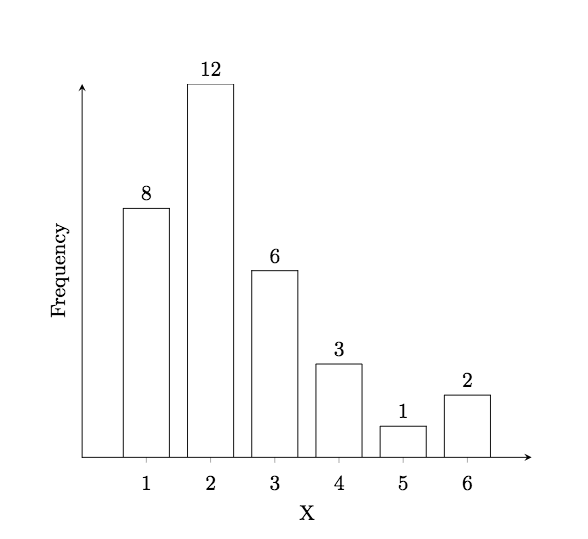
Consider the data set given by

🔗

Table 1.8.1. Basic Frequency Table

$x_k$	$f_k$
1	8
2	12
3	6
4	3
5	1
6	2

🔗

A frequency histogram representing this data looks like

🔗

Experiment with creating your own histogram by inputting your data into the interactive Sage cell below.

xxxxxxxxxx
 
#  This function is used to convert an input string into separate entries
def g(s): 
    S = str(s).replace(',',' ').replace('(',' ').replace(')',' ').split()
    return S
​
@interact
def _(freq = input_box("1,1,1,1,2,2,2,3,3,3,3,1,5",
                       label="Enter data separated by commas",
                      width=60)):
    freq = g(freq)
    freq = [int(k) for k in freq]
    m = min(freq)
    M = max(freq)
    bn = M-m+1
    histogram( freq, range=[m-1/2,M+1/2], bins = bn, align="mid", 
              linewidth=2, edgecolor="blue", color="yellow").show()

🔗

Relative Frequency Histograms - In this case, area describes relative frequency. Notice in the interactive cell above that each bar is of width one. Therefore, frequency = area. In some instances where data may be grouped the total width of the interval may be different and so the height will need to be adjusted so that the total area of each bar corresponds to the relative frequency of that category.

🔗

Cummulative Histograms. In these a running total is presented using all values from the given point and below.

xxxxxxxxxx
 
#  This function is used to convert an input string into separate entries
def g(s): 
    S = str(s).replace(',',' ').replace('(',' ').replace(')',' ').split()
    return S
​
@interact
def _(freq = input_box("1,1,1,1,2,2,2,3,3,3,3,1,5",label="Data separated by commas")):
    freq = g(freq)
    freq = [int(k) for k in freq]
    top = len(freq)
    m = min(freq)
    M = max(freq)
    bn = M-m+1
    histogram( freq, range=[m-1/2,M+1/2], cumulative = "true", bins = bn, 
              align="mid", linewidth=2, edgecolor="blue", color="yellow").show(ymax=top)

🔗

A Stem and Leaf Plot allows you to create a histogram of sorts but maintain the individual data values. To create one of these plots, you will need to consider your particular data set and create a two-step sieve for organizing the set. The first part is to create "stems" that are often associated with the highest digit(s) of each data value and the "leaves" that are often associated with the remaining digit(s) of the data value.

🔗

Once the data set is broken down into stems and leaves, it is often simple to sort the leaves under each stem to yield an "ordered Stem and Leaf Plot". Such as mechanism is a simple two-step procedure that allows you to sort a data set by hand.

🔗

Example 1.8.2. Simple Stem and Leaf Plot.

Consider the data points 25, 3, 17, 12, 22, 34, 12, 11, 16, 42, 9, 12, 17. In this case we will consider the stems to be the tens digits and the leaves to be the ones digits. This gives

Table 1.8.3. Stem and Leaf Plot (unordered)

Stems	Leaves
0	3 9
1	7 2 2 1 6 2 7
2	5 2
3	4
4	2

Then, an ordered Stem and Leaf Plot would be

Table 1.8.4. Stem and Leaf Plot (ordered)

Stems	Leaves
0	3 9
1	1 2 2 2 6 7 7
2	2 5
3	4
4	2

Notice, in each case you can extract the original data values by recombining the stem with a corresponding leaf. Indeed, for these 13 data values the median should be be 7th in the sorted list or the value in the 10's stem with leaf 6...that is, 16.

🔗

Example 1.8.5. Stem and Leaf Plot for State Populations.

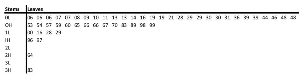
Using the state population data above, consider organizing the data but using a "two-pass sort" where you first roughly break data up into groups based upon ranges which relate to their first digit(s). In this case, let's break up into groups according to populations corresponding to 0-4 million, 5-9 million, 10-14 million, 15-19, million, 20-24 million, 25-29 million, 30-35 million, and 35-39 million. We can represent these classes by using the stems 0L, 0H, 1L, 1H, 2L, 2H, 3L, and 3H where the L and H represent the one's digits L in {0, 1, 2, 3, 4} and H in {5, 6, 7, 8, 9}. Once we group the data into these smaller groups then we can write the remaining portion of the number horizontally as leaves (in this case with one decimal place for all values.) This gives a step-and-leaf plot. If we additionally sort the data in the leaves then this gives you an ordered stem-and-leaf plot. For the state population data, the ordered stem-and-leaf plot is given by

Notice how it is easy to now see that most state populations are relatively small and that there are relatively few states with larger population. Also, notice that you can use this plot to relatively easily identify minimum, maximum, and other order statistics.

🔗

This graphical display identifies the 5-number-summary 1.3.14 associated with the minimum, quartiles 1.3.9, and the maximum. That is,

$y_1, Q_1, Q_2, Q_3, y_n\text{.}$ These values separate the data roughly into quarters. To distinguish these quarters connect

$y_1$ and

$Q_1$ with a straight line (a whisker) and do the same with

$Q_3$ and

$y_n\text{.}$ Use a box to connect

$Q_1$ with

$Q_2$ and the same to connect

$Q_2$ with

$Q_3\text{.}$ Then the boxed areas also identify the IQR.

🔗

xxxxxxxxxx
 
data <- c (0.6,0.6,0.6,0.7,0.7,0.8,0.9,1,1.1,1.3,1.3,
1.4,1.6,1.9,1.9,2.1,2.8,2.9,2.9,3,3,3.1,
3.6,3.9,3.9,4.4,4.6,4.8,4.8,5.3,5.4,5.7,
5.9,6,6.5,6.6,6.6,6.7,7,8.3,8.9,9.8,9.9,
10,11.6,12.8,12.9,19.6,19.7,26.4,38.3)
paste("Inter Quantile Range =",IQR(data))
paste("Box and Whisker Diagram - Box Plot):")
boxplot(data, horizontal=TRUE)

🔗

Essentials of Mathematical Probability and Statistics

Section 1.8 Visual Statistical Measures - Graphical Representation of Data

Example 1.8.2. Simple Stem and Leaf Plot.

Example 1.8.5. Stem and Leaf Plot for State Populations.

Checkpoint 1.8.6. WeBWorK - Computing Percentiles.