Notes on Linear Progarmming

Notes on Linear Programming

Dr. John Travis

(Adapted from http://ford.ieor.berkeley.edu/riot/Tools/InteractLP/)

Linear optimization consists in trying to find the optimal value (maximal or minimal value, depending on the problem) of a linear function of a certain number of variables (usually labeled x₁, x₂, ...x_n), given a set of m linear constraints on these variables (equalities or inequalities).

Even if it may seem quite theoretical in a first approach, linear optimization has a lot of practical applications in real problems. Especially, it is often used in industry, governmental, organizations, ecological sciences...to minimize objectives functions (that can be production costs, numbers of employees to hire, quantity of polluants relessed) given a set of constraints (availability of workers, of machines, ...).

Linear programming consists in solving the linear problems mentioned above, and developing the algorithms and software able to find the optimal solution to a problem, if there is one, or to prove that no solution exists if that is the case.

Each problem in Linear Optimization can differ in terms of the objective function (the objective can be either to minimize or maximize a function), as well as in terms of the linear constraints (equality constraints, inequality constraints, smaller or equal, strictly smaller...). The Linear Program is then usually converted into its standard form.

The generic linear program is formulated as follows:

Minimize c₁x₁ + c₂x₂ +.....+ c_nx_n (Objective function)

Subject to:

1st constraint:	a_1,1x₁+	a_1,2x₂+	....+	a_1,nx_n=	b₁
2nd constraint:	a_2,1x₁+	a_2,2x₂+	....+	a_2,nx_n=	b₂
...	...	...	...	...	...
...	...	...	...	...	...
m-th constraint:	a_m,1x₁+	a_m,2x₂+	....+	a_m,nx_n=	b_m

Positivity:	x₁>0	x₂>0	...	x_n> 0

Or, using vectors and matrices:

Min CX
Subject to:
where X > 0
and C such that	(c₁, c₂, ...c_n)

Conversions needed:

Conversion of "less than" inequalities into equalities.
Conversion of "greater than" inequalities into equalities.
Non positive variables.
Maximization problems.

Conversion of "less than" inqualites to equalities

Suppose that the k^th constraint is a smaller than equality labeled as follows:

a_k,1x₁+a_k,2x₂+... +a_k,mx_m< b_k

It is equivalent to say that, for some value x_m+1, a_k,1x₁+a_k,2x₂+... +a_k,mx_m+x_m+1=b_k

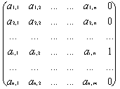
where x_m+1, is a positive variable know as a slack variable. So, we must consider a new column-vector X=(x₁, x₂, ... , x_n )^t. To incorporate this into the original problem, add a column to matrix A with zeros everywhere except on the k^th line (where we will put a 1, so as to include the x_m+1 in the k^th constraint), so that A becomes:

Further, we must add a column to vector C (simply one zero, since the new slack variable, x_m+1, must not affect the value of the objective function) so that C becomes (c₁, c₂, ..., c_n, c_n+1) where c_n+1=0.

So we have a new problem, with the same n constraints, but m+1 variables. If we repeat this process with all the "smaller than" inequalities, and introduce one slack variable for each of them, then we obtain a new problem where all the "smaller than" inequalities are replaced by equalities.

Conversion of "greater than" inqualites to equalities
Suppose that the k^th constraint is a bigger than equality labeled as follows:

a_k,1x₁+a_k,2x₂+... +a_k,mx_m>b_k It is equivalent to say that, for some value x_m+1, a_k,1x₁+a_k,2x₂+... +a_k,mx_m-x_m+1=b_k with x_m+1 a positive slack variable. Proceed in a manner similar to above to modify A and C.

Conversion of non-positive variables

You have certainly noticed that the standard formulation of a linear program is quite restrictive, since it does only consider positive variables. In reality, it does not constitute a problem, since we can easily convert a problem where some variables are not required to be positive into a problem with only positive variables.

Indeed, suppose that the k^th variable x_k has no positivity constraint. We the introduce two "artificial variables": x'_k and x''_k and replace x_k by x_k = x'_k - x''_k. So, we can still have x_k either positive or negative, with x'_k and x''_k positive. The new variable column-vector is

(x₁, x₂, ... , x'_k, x''_k, ... , x_n )^t. where x'_k and x''_k positive.

This duplication of variable x_k into two variables obliges us to update matrix A and vector C:

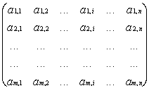
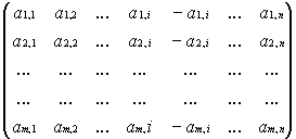
In matrix A, we add a new column labeled A'_.,i between columns k and k+1, equal to the opposite of the original column k. So A, that was equal to

_k,j

For vector C, we introduce a number c'_k between c_k and c_k+1 with c'_k = -c_k , so that :

₁

₂

x_k = x'_k - x''_k

Maximization Problems

You have certainly noticed that the standard formulation of a linear program is quite restrictive, since it only considers minimization problems. In reality, it does not constitute a problem, and it is very easy to convert a maximization problem into a minimization problem.

Indeed, suppose that your problem is: Maximize c₁x₁ + c₂x₂ +.....+ c_nx_n (Objective function)
This is strictly equivalent to: Minimize -c₁x₁ - c₂x₂ -.....- c_nx_n
and take the opposite of the optimal value of the objective function for this minimization problem as the optimal value for the original (maximization) problem.
So, what you only need to do is:

Take the opposite of vector C. That is use (-c₁ ,-c₂ ,... ,-c_n).
Solve the standard linear program minimize (-C)X, subject to the same constraints as the original problem.
Take the opposite of the result as the optimal value of the objectif function for the original problem, and the same values of the variables x₁ ,x₂ ,... ,x_n as the optimal solution.

HOW TO SOLVE THE LINEAR PROGRAMMING PROBLEM

Geometric Solution - Can be performed if the problem is 2 dimensional
Simplex Method

Geometric Solution: Since the constraints are all linear expressions, graph the boundaries of these constraints and create a "feasible region" in the plane. Identify all corners of this feasible region. Draw the (linear) objective function for some point in the feasible region and note that this corresponds to a "level curve" of all values in the feasible region which all have the same value for the objective function. Then, to minimize the objective function, determine which direction give level curves with smaller values until you arrive at one of the endpoints.

Theorem 9.1: Suppose the feasible region of a linear program is a nonempty and bounded convex set. Then, the objective function must attain both a maximum and minimum value occurring at extreme points of the region. If the feasible region is unbounded, the objective function need not assume its optimal values. If either a maximum or minimum does occur, it must occur at one of the extreme points.

HOMEWORK: page 310 #2, 4

Simplex Method: As above, first convert all inequalities to equalities by using slack variables and all variables to non-negative variables using artificial variables, if needed. Consider the set of original variables as comprising the independent set and the slack variables as comprising the dependent set.

STEPS:

Arrange the equations into a "Tableau"
Start with an initial extreme point, usually at the origin
Determine whether an adjacent intersection point improves the value of the objective function. If so, update.
Eliminate one of the variables in the dependent set thus determing one of the independent sets variables (and thus making that variable dependent.)
Form a new equivalent system of equations by eliminating the new dependent variable created in the previous step from all other equations that contain that variable
Repeat until an optimal extereme point is found.

Sensitivity Analysis:

THE BASIC CERTIFICATES

When you try to solve a problem in linear optimization, one thing that you would usually like to do is to prove that your conclusions are true, i.e that your problem is really infeasible, or unbounded, or that the optimal solution that you propose is really optimal. In order to do that, the theory of linear programming provides us for some equations that are likely to prove these three possible conclusions. These equations, if we solve them (i.e find some vectors Y or U or W that satisfy them, as you will see later on) prove that our conclusions are true. They are called the basic certificates.

Certificate of Infeasibility

The certificate of infeasibility consists in one (1*n) row-vector Y such that:

Y * A < 0.
Y * B > 0.

Indeed, if there existed any feasible vector X solution to the problem (i.e. a vector X such that A*X=B, X > 0) then for any vector Y satisfying inequality (1.), we would have:

Y*A < 0
=> (Y*A)*X < 0 (since X> 0)
=> Y*B < 0 (since A*X = B)
=> no vector Y that verifies (1.) can verify (2.).

Certificate of Unboundedness

The unbondedness certificate consists in:

Vector X (a (m*1) column-vector).
Vector W (a (m*1) column-vector).

These two vectors are such that:

A*X = B.
X > 0.
A*W = 0.
W > 0.

Indeed, 1/ and 2/ guarantee that X is a feasible solution to the problem. 3/ guarantees that, for any number l>0, X + l*W is still a feasible solution, since:

A*[X+(l*W)] = A*X + l*(A*W) = B+0 = B.
X+(l*W) > 0 (since W, X and l > 0).

Last, 4/ guarantees that, if we choose l large enough, we can find a feasible solution (equal to X+lW) that gives a value of the objective function as small as we want (since C * (X+lW) = (C*X) + l(C*W), with C*W < 0 and l > 0, as large as we want.

Certificate of Optimality

The certificate consists of:

Vector X (the optimal solution, a m-column-vector).
Vector Y (a n-row-vector).

These two vectors are such that:

A*X = B
X > 0.
Y*A < C.
[C-(Y*A)]*X = 0.

Indeed, 1/ and 2/ guarantee that X is a feasible solution to the problem. 3/ Guarantees that for any feasible solution X, then C*X > Y*B (We obtain this result by multiplying 3/ by X and replacing, if X is a feasible solution, A*X by its value, i.e. B). So, Y*B is a lower bound on the value of the objective function for any feasible solution.
4/ guarantees that C*X = (Y*A)*X = Y*B = lower bound on the value of the objective function.
So, X is a feasible solution, and the value of the objective function for X is equal to the lower bound. Thus, X is an optimal solution.